ScanFields

After installting a cross-link databese saved in HDF5 format, we can load every infomation related with scanning strategy such as a hit-map and cross-link map. This information will be an object by sbm.ScanFields class. The following code snippet shows how to access the hit-map and cross-link map.

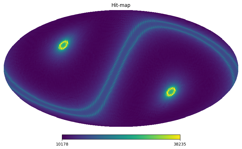
Hit-map

This is a code sample to access the hit-map:

import numpy as np
import healpy as hp
import matplotlib.pyplot as plt
import sbm
from sbm import ScanFields

test_xlink_path = "sbm/tests/nside_32_boresight_hwp.h5"
sf_test = sbm.read_scanfiled(test_xlink_path)
hp.mollview(sf_test.hitmap, title="Hit-map")
display(sf_test.ss)

{'alpha': 45.0,
'beta': 50.0,
'coord': b'G',
'duration': 31536000,
'gamma': 0.0,
'hwp_rpm': 61.0,
'name': array([b'boresight'], dtype=object),
'nside': 32,
'prec_rpm': 0.005198910308399359,
'sampling_rate': 5.0,
'spin_rpm': 0.05,
'start_angle': 0.0,
'start_point': b'equator'}

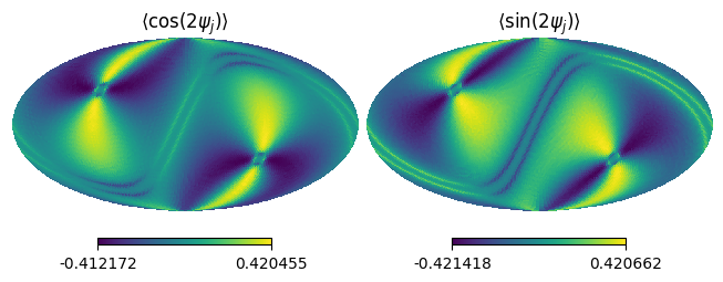
Cross-link

Also, we can access the cross-link map as follows:

xlink2 = sf_test.get_xlink(2, 0) # n=2, m=0
hp.mollview(xlink2.real, title=r"$\langle \cos(2\psi_j) \rangle$", sub=(1,2,1))
hp.mollview(xlink2.imag, title=r"$\langle \sin(2\psi_j) \rangle$", sub=(1,2,2))

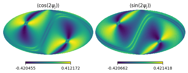
If we want to have a cross-link simulated by orthogonal pair detector, we can use ScanFields.t2b(). This method apply the exponential factor to rotate the phase of detector as:

\[{}_{n,m}\tilde{h}^{(\texttt{B})} = {}_{n,m}\tilde{h}^{(\texttt{T})}e^{i n \frac{\pi}{2}}.\]

xlink2 = sf_test.t2b().get_xlink(2, 0) # n=2, m=0
hp.mollview(xlink2.real, title=r"$\langle \cos(2\psi_j) \rangle$", sub=(1,2,1))
hp.mollview(xlink2.imag, title=r"$\langle \sin(2\psi_j) \rangle$", sub=(1,2,2))

Covariance matrix

By combining cross-links using ScanFields.create_covmat(), we can create covariance matrix to reconstruct signals. For instance, if we want to reconstruct the spin-0 and spin-2 field, we can use the following code snippet:

spin_n_basis = [0, 2, -2] # spin-n
spin_m_basis = [0, 0, 0]  # spin-m
C = sf_test.create_covmat(spin_n_basis, spin_m_basis)

C is a \(3\times3\times N_{\rm pix}\) numpy.ndarray though we can see the analytical covariance matrix \(C\) by

display(sf_test.model_covmat())

Output:

\[\begin{split}\left[\begin{matrix}1 & \frac{{}_{-2,0}\tilde{h}}{2} & \frac{{}_{2,0}\tilde{h}}{2}\\\frac{{}_{2,0}\tilde{h}}{2} & \frac{1}{4} & \frac{{}_{4,0}\tilde{h}}{4}\\\frac{{}_{-2,0}\tilde{h}}{2} & \frac{{}_{-4,0}\tilde{h}}{4} & \frac{1}{4}\end{matrix}\right]\end{split}\]